Simulated annealing
From DDL Wiki
Simulated Annealing (SA) is a multidimensional optimization method inspired by the metallurgical process of annealing. In metal, this is accomplished by heating a specimen and allowing the molecules to diffuse to more stable positions. As the temperature is slowly lowered the molecules settle to positions which result in lower internal stresses. The same general process is used in simulated annealing where a temperature value is assigned to the function, and the optimization occurs as that temperature drops.
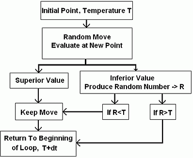
In the beginning of the algorithm a temperature value is assigned to the function and a starting point is defined. A random move is made away from the current position and the function is re-evaluated at this new point. If the new value is an improvement, this move is kept. If the new point produces a less desirable value then temperature comes into play. A randomly generated value (within the range of the maximum and minimum temperatures) is compared to the current temperature. If this random value is lower than the current temperature, the undesirable move is made anyway. Otherwise the move is ignored and the process repeats. This ability to make uphill moves allows the function to easily make its way out of local minima while the temperature is high yet makes undesirable moves unlikely as the temperature drops. In order for the function to terminate properly the temperature must decrease as time progresses. Therefore the temperature is reduced by a small value after each iteration.
Contents |
Moving
At the beginning of each iteration, a move is randomly made. Many methods can be used to make these moves including univariate steps; although it is generally better to change several variables with each step. The size of each step taken is also critical. Large step sizes are necessary so that the algorithm may efficiently approach desired values. Once the function approaches the global minima a smaller step size may then be necessary to produce a value close to the true minima. For this reason it can be beneficial to make the step size a function of temperature. By doing this large steps are made in the beginning operation but step size decreases as the system becomes more stable. Inclusion of this routine further reflects the similarity with metallurgical annealing. Molecules tend to move less and less as thermal energy decreases and intermolecular forces dominate the system.
Temperature
The temperature value will begin at a high value and end at a low value once the optimization is completed. The easiest way to implement this is to begin with a high temperature of 1.0, and end with a low temperature of zero. With each iteration the temperature will drop by some finite value.
In order for simulated annealing to work properly, the changes in temperature must fit the problem being analyzed. Allowing the temperature to change too quickly will not give the algorithm enough time to escape local minima properly. Setting the change too low will force the function to run longer than is necessary. Doing so is computationally inefficient and should be avoided if possible.
The rate at which the temperature changes, and the ending criteria are referred to as the annealing schedule.
Flow Chart
Strengths and Weaknesses
Simulated annealing algorithms can easily accommodate constraints because constraint values can easily be added onto the values evaluated at each move.
The main weakness of simulated annealing is that it is always possible to become stuck at local minima. This can be avoided to some extent through use of a proper annealing schedule and starting point.
External links
- Functional Minimization using Simulated Annealing A Fortran 90 code implements simple simulated annealing algorithm.
- Numerical Recipes The well-known numerical- method book talks about simulated annealing in Chapter 10.9.

