Ski boot walking attachment analysis
From DDL Wiki
(→Determination of Spring Constants and Damping Coefficients) |
(→Determination of Spring Constants and Damping Coefficients) |
||
| Line 12: | Line 12: | ||
<big>'''Overview of Method'''</big> | <big>'''Overview of Method'''</big> | ||
| - | In order to obtain values for the spring constant and damping coefficient of each material, we will use the rectilinear experimental setup used in the Mechanical Systems Experimentation lab. This setup, as pictured | + | In order to obtain values for the spring constant and damping coefficient of each material, we will use the rectilinear experimental setup used in the Mechanical Systems Experimentation lab. This setup, as pictured in the first thumbnail on the right, consists of carts attached to tracks with encoders used to measure displacement. We can attach the carts to a stationary post using springs, or, in this case, our materials. In order to find the spring constant and damping coefficient, we can manually move the carts and find the response. Using MATLAB code developed for our MSE labs, we can use the logarithmic decrement method to find the spring constants and damping coefficients. |
| - | In order to attach the materials to the rectilinear system, we had to specially design brackets to hold the materials and clamp on to the provided posts and carts. To do this, we used the system pictured | + | With logarithmic decrement, the damping ratio is obtained with the following formula, where n = number of peaks used, x<sub>1</sub> = the displacement on the first peak, x<sub>n</sub> = displacement on the ''n''th peak, and zeta = damping ratio. |
| + | [[Image:SkiBoot_LogarithmicDecrement.jpg|center]] | ||
| + | |||
| + | Using the damping ratio, we can obtain the natural frequency with the following formula, where T = period, omega = natural frequency, and the rest of the variables have the same definitions as above. | ||
| + | [[Image:SkiBoot_NaturalFrequency.jpg|center]] | ||
| + | |||
| + | Using the natural frequency, we can find the spring constant using the following formula, where k = spring constant and the rest of the variables have the same definitions as above. | ||
| + | [[Image:SkiBoot_SpringConstant.jpg|center]] | ||
| + | |||
| + | Using the damping ratio and spring constant, we can obtain the damping coefficient using the following formula, where b = damping coefficient, zeta = damping ratio, k = spring constant, and m = mass. | ||
| + | [[Image:SkiBoot_DampingRatio.jpg|center]] | ||
| + | |||
| + | Additionally, we can check our results for the spring constants by using a ramp function input and the dividing the input force by the displacement response over the course of the run. With these two tests run together, we can get at least some idea of the spring constant, and with just the one test we can get some somewhat accurate idea of the damping coefficient. | ||
| + | |||
| + | In order to attach the materials to the rectilinear system, we had to specially design brackets to hold the materials and clamp on to the provided posts and carts. To do this, we used the system pictured in the bottom two thumbnails on the right. In the first picture, you can see the completed bracket with the material already screwed inside. The material is placed in the clamp-like area between the two pieces of acrylic. We then run screws through the acrylic, through the material, and out the other piece of acrylic to create a tight hold on the material. One piece of the acrylic is then attached to the stationary post on the rectilinear setup using the large screw sticking out of the back. The other piece of acrylic is mounted to the cart using the large screw. Since we couldn't find properly sized screws, we have implemented a couple nuts to hold the screw in the proper position. | ||
<big>'''Assumptions Made'''</big> | <big>'''Assumptions Made'''</big> | ||
Revision as of 18:44, 10 November 2008
Brandon
Taka
Determination of Spring Constants and Damping Coefficients
Purpose of the Analysis
We are doing this analysis to obtain at least ballpark figures for the spring constant and damping coefficient of each of the materials we will be using to construct the body of our walking attachment. These are important because they allow us to actually have numbers instead of vague ideas about how well the materials act as springs and dampers. In addition, Taka and Brandon need some kind of ballpark values in order to make their analyses more accurate and more useful.
Overview of Method
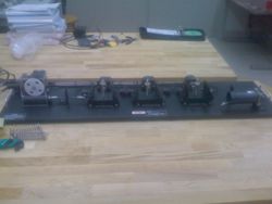
In order to obtain values for the spring constant and damping coefficient of each material, we will use the rectilinear experimental setup used in the Mechanical Systems Experimentation lab. This setup, as pictured in the first thumbnail on the right, consists of carts attached to tracks with encoders used to measure displacement. We can attach the carts to a stationary post using springs, or, in this case, our materials. In order to find the spring constant and damping coefficient, we can manually move the carts and find the response. Using MATLAB code developed for our MSE labs, we can use the logarithmic decrement method to find the spring constants and damping coefficients.
With logarithmic decrement, the damping ratio is obtained with the following formula, where n = number of peaks used, x1 = the displacement on the first peak, xn = displacement on the nth peak, and zeta = damping ratio.
Using the damping ratio, we can obtain the natural frequency with the following formula, where T = period, omega = natural frequency, and the rest of the variables have the same definitions as above.
Using the natural frequency, we can find the spring constant using the following formula, where k = spring constant and the rest of the variables have the same definitions as above.
Using the damping ratio and spring constant, we can obtain the damping coefficient using the following formula, where b = damping coefficient, zeta = damping ratio, k = spring constant, and m = mass.
Additionally, we can check our results for the spring constants by using a ramp function input and the dividing the input force by the displacement response over the course of the run. With these two tests run together, we can get at least some idea of the spring constant, and with just the one test we can get some somewhat accurate idea of the damping coefficient.
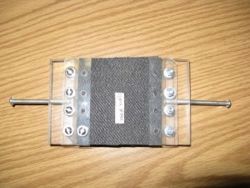
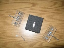
In order to attach the materials to the rectilinear system, we had to specially design brackets to hold the materials and clamp on to the provided posts and carts. To do this, we used the system pictured in the bottom two thumbnails on the right. In the first picture, you can see the completed bracket with the material already screwed inside. The material is placed in the clamp-like area between the two pieces of acrylic. We then run screws through the acrylic, through the material, and out the other piece of acrylic to create a tight hold on the material. One piece of the acrylic is then attached to the stationary post on the rectilinear setup using the large screw sticking out of the back. The other piece of acrylic is mounted to the cart using the large screw. Since we couldn't find properly sized screws, we have implemented a couple nuts to hold the screw in the proper position.
Assumptions Made
In using the same kind of analysis we used in our MSE lab, we have assumed that the springs are linear. This may or may not be the case with the materials that we are testing. In order to correct for this, we will make sure to do each test a few times using different conditions. If the values match up pretty well, we can say that our assumption of a linear spring is valid. If the values don't match up well, our assumption is probably not valid, but it doesn't make the analysis completely pointless. Even if we can't get very exact values for the spring constant and damping coefficient, we still at least can get ballpark values, which is really what we want. Since no other tool of analysis we are using is especially accurate, we just need approximate spring constants and damping coefficients. In addition, a major purpose of this analysis is to acquire the spring constants and damping coefficients relative to each other. Whether or not the obtained values are particularly accurate is of minimal consequence.
Our assumptions also exclude the effects of friction, which there will obviously be. Again, since we are not looking for exact values for the material properties, this is of little consequence. As long as we obtain material properties on the right order of magnitude, Brandon and Taka should be able to run their analyses with a fair amount of accuracy. Since the other purpose of this analysis is to help us decide how to layer the sheets of rubber and foam, we only need relative values for.


