From DDL Wiki

After collecting the feedbacks from users, who tested out the Prototype I, we concluded that the alternating layers of various rubber materials appear to improve a walking motion in ski boots. Therefore, the main goal of this "design memo" is to justify the use of alternating layers of different materials as opposed to using a large blocks of single material for walking attachment soles. The analyses consist of three major components - improvement of Matlab code, simple beam model analyses using manual calculations and FEA, and determination of effective spring stiffness of each rubber sample. Improvement of Matlab code will allow calculation of the optimal stress distribution on users' feet, while FEA would help establish the combination of rubber materials that yields the desired stress distribution. Finally, determination of spring stiffness of rubber materials is essential for manufacturing the optimal design calculated by the FEA. Since the access to Mechanical System Experimental Laboratory apparatus has not been available, the physical properties of rubber materials are yet to be determined; however, the simple beam analyses display that alternating layers of various spring elements is an effective method for achieving the desired stress distribution.

Simple Beam Model Analysis

Theoretical Model

Purpose of the Analysis

The primary goal of the simple beam model analyses using the theoretical model is to justify the use of layers of various rubber materials as an effective method of adjusting the net effective spring constant of specific region of the walking attachment.

Overview of Method

The theoretical model consists of several linear springs with various stiffness aligned in parallel. The theoretical model is prefered when predicting the static deformation of the walking attachment's soles. Under these simulations, only a vertical load is applied through the layers of rubber materials, and each segment of the sole can be treated as a linear spring.

The fundamental equation of the relationship between the displacement of linear springs in parallel and the external force being applied is listed below:

k_effective = k₁ + k₂ + ... k_n

The theoretical model is more reliable than Finite Element Analysis (FEA) when the analysis is simple and no tangential force is present. This is because the FEA requires setting the mesh size to an adequate level in order to obtain accurate results, and often times, stress concentration around sharp edges tends to approach infinity (which does not occur in reality). The theoretical model is simple, yet accurate enough for predicting the overall effective spring coefficient of the layers of rubber material as long as only vertical load is applied, and the deformation is reasonablly small. If friction force between the ground and the bottom of the walking attchment needs to be included in the analyses, the model will not satisfy the assumption that each segment of rubber material behaves as a linear spring due to the moment created by the tangential force. Also, when the significant amount of deformation occurs, behaviors of physical springs tend to diverge from that of ideal springs.

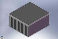
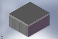
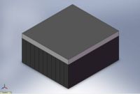
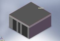
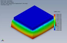
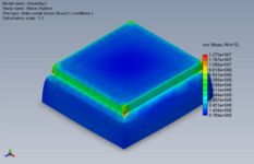
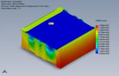
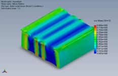
Following are the four simple models, whose net effective spring stiffness is calculated using the equation mentioned above. Each of those models are also designed and tested during the FEA (which is summarized in the next chapter). Images of those simulation models are available in the next chapter (Simple Beam Model Analyses - FEA) as well.

(1) To simulate the regions, where materials with high and low spring stiffness are altered, six layers of silicon (high stiffness material in this model) and five layers of rubber (low stiffness material in this model).

(2) To simulate the high stiffness region, a model that has silicon as all eleven of its spring elements was tested.

(3) To simulate the low stiffness region, a model that has rubber as all eleven of its spring elements was tested.

(4) To simulate the effect of varying the thickness of silicon layers and rubber layers, a model with Si-Si-Ru-Ru-Si-Ru-Si-Ru-Ru-Ru-Si combination was tested.

Assumptions and Boundary Conditions

• Treat each layer of rubber material as a linear spring element

• Only vertical load is being applied to the layers of rubber materials
  • As mentioned above, the theoretical model is accurate only when the rubber materials do not experience shear forces. Shear forces would cause spring elements' horizontal displacement, and rubber materials would no longer behave as linear spring elements.

• The user stands on a completely flat surface
  • Each spring element experiences the same amount of vertical deformation
  • This assumption is used just to simplyfy the analyses. If the deformation of the walking attachment's sole while the user walks on a slope needs to be determined in future analyses, it is likely that the FEA will be the primary method.

• The deformation of the spring element is small enough
  • If the vertical load compresses the rubber materials too far away from its equillibrium position, the physical springs' behaviors may diverge from that of ideal springs.

• Let the effective stiffness of each layer of rubber be 1N/mm and that of Si be 10N/mm
  • The spring coefficients of every rubber material will be obtained using MSE lab experiment apparatus.
  • For the time being, let the effective stiffness of the rubber be one tenth of the stiffness of Si to simplify the calculation.
  • In the next section (FEA), SolidWorks material properties (stored in the software's library) of rubber and Si are used to simulate the model.

Conclusions

The calculations yield the net spring stiffness of each model to be...

Model 1: 1.964 N/mm [Si-Ru-Si-Ru-Si-Ru-Si-Ru-Si-Ru-Si] Model 2: 10.000 N/mm [All Si] Model 3: 1.000 N/mm [All Rubber] Model 4: 1.692 N/mm [Si-Si-Ru-Ru-Si-Ru-Si-Ru-Ru-Ru-Si]

These calculation results will be compared against the results of FEA discussed in the next chapters. One thing to be noted is that teh calculation results from this theoretical model does not reflect any change in allocation of Si and Rubber layers. The net effective spring stiffness is only the function of the number of Si layers and number of Rubber layers that consist the model.

Finite Element Analyses (FEA) of a CAD (SolidWorks) model

1st model consists of alternating pattern of Si and Rubber layers.

2nd model consists of one large Si layer.

3rd model consists of one large Rubber layer.

4th model consists of Si-Si-Ru-Ru-Si-Ru-Si-Ru-Ru-Ru-Si combination.

Purpose of the Analysis

There are two primary goals of the simple beam model analyses using FEA.

(1) To justify use of layers of various rubber materials as an effective method of adjusting the effective spring constant of specific region of the walking attachment (just like the primary purpose of the theoretical model analyses).

(2) To determine the change in stress distributions as the combinations of rubber materials vary

Overview of Method

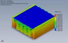
The SolidWorks model consists of a 10cm x 11cm base made of aclylic and eleven 10cm x 1cm x 5cm spring element layers made of various materials. Four combinations of spring elements were simulated to undergo 1cm of uniform compression in vertical direction while the base plate was being fixed.

(1) To simulate the regions, where materials with high and low spring stiffness are altered, six layers of silicon (high stiffness material in this model) and five layers of rubber (low stiffness material in this model).

(2) To simulate the high stiffness region, a model that has silicon as all eleven of its spring elements was tested.

(3) To simulate the low stiffness region, a model that has rubber as all eleven of its spring elements was tested.

(4) To simulate the effect of varying the thickness of silicon layers and rubber layers, a model with Si-Si-Ru-Ru-Si-Ru-Si-Ru-Ru-Ru-Si combination was tested.

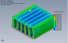
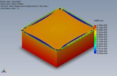
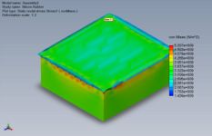
Each model experiences uniform 1cm vertical compression while the base plate is "fixed." Both the displacement (deformation) and stress distributions plots are obtained from each simulation, and the net reaction forces in the vertical reaction (which is the force needed to cause the simulated deformation of spring elements) are also calculated.

Assumptions and Boundary Conditions

• Treat silicon layer as a high stiffness and rubber layer as a low stiffness spring element
  • Only two types of spring elements are used to simplify the analyses and focus on the effects of layer combinations and layer thickness on the effective stiffness of the entire model.

• Only vertical load is being applied to the layers of rubber materials
  • The primary goal of this analsis is "to justify the use of layers of various materials as an effective method for adjusting the effective spring stiffness."

• Each spring element experiences the same amount of vertical deformation (1cm)
  • If the load gets uniformly distributed over the bottom surface of the walking attachment, rubber layers (low stiffness spring elements) would deform more than silicon layers (high stiffness spring elements) do. In reality, however, the vertical force is applied on the spring elements via contact with the ground. Therefore, the deformation of the bottom surface (rather than the distribution of the load) needs to be uniform.

Conclusions

As predicted by much simpler theoretical models (in the previous chapter), displacement plots of simulations 1 and 4 display similar results. Also, the model 2 (All Si - high stiffness spring element) experiences much greater stress as its net effective spring stiffness is much greater than any other model, and to experience 1cm of vertical compression, much greater normal force (which linearly correlates to von Mises stress shown in the stress plot) needs to be applied.

The stress plots are also used to address the conclusion for the primary goal of this analysis - The use of alternating layers of various spring elements is an effective method for optimizing the walking attachment's design. As summarized in the stress plots of simulations 1 and 4, high stiffness spring elements (Si layers) experience much greater von Mises stress than low stiffness spring elements (Rubber layers) do. Thus, the FEA proves that using alternating layers of spring elements with various stiffness would effectively alter the stress distribution inside the sole of the walking attachment. Therefore, once the desired stress distribution experienced by user's feet is determined by the matlab simulation code, and the physical experiment results reveal spring stiffness per cross sectional area of each rubber material, the optimal design for the walking attachment can be calculated.

Model 1 Results: Alternating Layers

Simulation 1 Displacement.

Simulation 1 Stress.

Model 2 Results: All Silicon Layers

Simulation 2 Displacement.

Simulation 2 Stress.

Model 3 Results: All Rubber Layers

Simulation 3 Displacement.

Simulation 3 Stress.

Model 4 Results: Si-Si-Ru-Ru-Si-Ru-Si-Ru-Ru-Ru-Si

Simulation 4 Displacement.

Simulation 4 Stress.

Determination of Spring Constants and Damping Coefficients

Purpose of the Analysis

Rectilinear system used to test material properties.

Mount with material inside.

Mount and material taken apart with screw used to put material in mount.

The goal of this analysis is to obtain reasonablly accurate spring constant and damping coefficient of each of the rubber materials being used for construction of the walking attachment. These experiments are essential for optimization of the walking attachment design since they would provide us with quantitative measures of the material properties as opposed to vague ideas of how well the materials act as springs and dampers. In addition, the material properties obtained in this experiment are crucial for beam model and MATLAB analyses in order for them to be more intuitive. Especially, providing the MATLAB model with accurate data would help determine the optimal compositions of rubber and foam (neoprene, silicone, or natural rubber).

Overview of Method

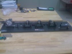
In order to obtain the spring constant and damping coefficient of each material, the rectilinear experimental apparatus for the Mechanical Systems Experimentation (MSE) lab (24452) will be used. This apparatus, as displayed in the first thumbnail on the right, consists of a motor, three carts, vertical supports, and three encoders. The motor applies inputs specified by the experimenters, the encoders measure the displacements, velocity, and acceleration of each cart. The carts can be connected to the vertical supports by springs or in this case, various rubber and foam samples. In order to determine the spring constant and damping coefficient, initial displacement from the equillibrium position can be applied manually, and the carts' response will be monitored. Using MATLAB code developed for the MSE labs, the logarithmic decrement method will calculate the spring constants and damping coefficients.

With logarithmic decrement, the damping ratio is obtained with the following formula, where n = number of peaks used, x₁ = the displacement on the first peak, x_n = displacement on the nth peak, and zeta = damping ratio.

Using the damping ratio, we can obtain the natural frequency with the following formula, where T = period, omega = natural frequency, and the rest of the variables have the same definitions as above.

Using the natural frequency, we can find the spring constant using the following formula, where k = spring constant and the rest of the variables have the same definitions as above.

Using the damping ratio and spring constant, we can obtain the damping coefficient using the following formula, where b = damping coefficient, zeta = damping ratio, k = spring constant, and m = mass.

In addition to the initial displacement tests, applying a ramp input and dividing the input force by the displacement response over the course of the run could yield another measure for the material properties. With results from the two tests, reasonablly accurate values of the spring constant and the damping coefficient can be obtained.

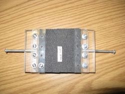
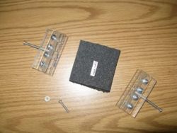
In order to attach the materials to the rectilinear apparatus, we had to specially design brackets to hold the materials and clamp on to the provided posts and carts. To do this, we used the system pictured in the bottom two thumbnails on the right. In the first picture, you can see the completed bracket with the material already screwed inside. The material is placed in the clamp-like area between the two pieces of acrylic. We then run screws through the acrylic, through the material, and out the other piece of acrylic to create a tight hold on the material. One piece of the acrylic is then attached to the stationary post on the rectilinear setup using the large screw sticking out of the back. The other piece of acrylic is mounted to the cart using the large screw. Since we couldn't find properly sized screws, we have implemented a couple nuts to hold the screw in the proper position.

Assumptions Made

In using the same kind of analysis we used in our MSE lab, we have assumed that the springs are linear. This may or may not be the case with the materials that we are testing. In order to correct for this, we will make sure to do each test a few times using different conditions. If the values match up pretty well, we can say that our assumption of a linear spring is valid. If the values don't match up well, our assumption is probably not valid, but it doesn't make the analysis completely pointless. Even if we can't get very exact values for the spring constant and damping coefficient, we still at least can get ballpark values, which is really what we want. Since no other tool of analysis we are using is especially accurate, we just need approximate spring constants and damping coefficients. In addition, a major purpose of this analysis is to acquire the spring constants and damping coefficients relative to each other. Whether or not the obtained values are particularly accurate is of minimal consequence.

Our assumptions also exclude the effects of friction, which there will obviously be. Again, since we are not looking for exact values for the material properties, this is of little consequence. As long as we obtain material properties on the right order of magnitude, The MATLAB model and the beam model analyses should be able to be conducted with a fair amount of accuracy. Since the other purpose of this analysis is to help us decide how to layer the sheets of rubber and foam, we only need relative values for.

Conclusions

Though the necessary materials, clamps, and theory are ready for experimentation, approval from the laboratory is pending. As soon as this permission is granted, testing will be completed and dynamic properties will be available for integration into the MATLAB model and the simple beam model.

MATLAB Model

Purpose

The premise of the revised walking attachment is to improve comfort, control, and general walking ability. Intuition generated the first ideas regarding the chosen order of foam and rubber layers; the next step in the optimization is computer modeling. Using this MATLAB model, the ideal damping and spring amounts, locations, and zones can be determined by fitting the model output with the theoretical ideal step.

Assumptions

• Constant forward body velocity, and .6 seconds of foot contact per step
• Ideal hip motion is harmonic
• Expected hip motion is similar to the ski boot with no device attached
• Ankle is locked
• All deflection is one-dimensional, and normal to sole of foot
• All forces are exerted vertically
• Ideal spring-damping setup

Existing Model Data

Appendages included in simulation

Though it was obvious from simply wearing the ski boots that the step was changed, the specific change was not understood.

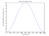
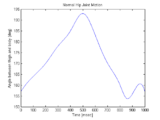
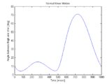
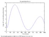
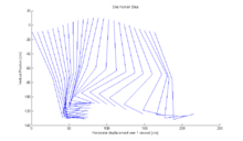
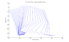
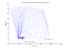
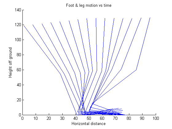
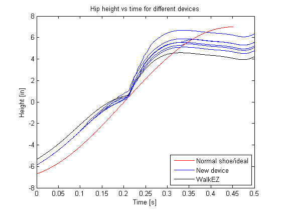
To address this lack of knowledge, a simulation was written in MATLAB to calculate foot, leg, and body motion during three step variations. A normal step is provided as a reference; the bare ski boot step demonstrates the roughness of the gait; and, finally, the efficacy of the WalkEZ is shown very clearly. The attachment eliminates the roughness created by the locking of the ankle, though the step is not restored to its original geometry.

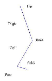
The model employs kinesiologic research of joint motion in steps as described by Soutas-Little (cf references). For the normal gait, assumptions include standard footwear on an able person at a comfortable walking pace. To simulate a user wearing a ski boot, the ankle ankle is locked in the simulation, though other joint motion remains the same. Constant forward torso velocity is still assumed, and experimental results are consistent with this assumption. To simulate the WalkEZ, the entire leg is raised and lowered as the WalkEZ 'rolls' as it contacts the ground at the same angle as the foot. The simulation output is a diagram of limb position with respect to time. Joint motion data (as shown below) and with average limb lengths are the input, along with factors such as a locked ankle and the presence of a WalkEZ. Further customization is not implemented at this time, as the current level of control provides the desired function.

Cubic splines were fitted in MATLAB to provide continuous data for the simulations.

The results of this simulation are an analytical validation of the problem and current solution and are immediately useful as such. Additionally, future usefulness may be incalculable, as simulation of proposed designs will be possible with relevant additions to the code.

Normal Step

Hip height change during step.

Hip flex during step (torso-thigh angle)

Knee flex during step (thigh-shin angle)

Ankle flex during step (shin-foot angle)

Simulation of normal step motion

Simulation of step wearing ski boot

Simulation of step wearing ski boot and walking device

Effect of footwear selection upon Center of Mass change during stride. Note the attachment greatly smooths the change while the foot is bearing the body's weight.

As shown above, the device provides a significant improvement to the smoothness of the step, though it is only a partial solution. Further work is necessary to make the gait even more natural.

Method

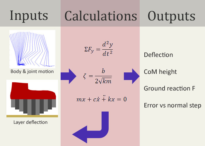
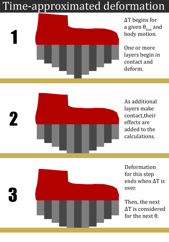
The model uses time-stepping and binning to make calculations reasonable.

The analysis flows as such:

• A layer or layers of the device (for the first t, the heel) contacts the ground
• That layer(s) undergoes deformation until either:
  • the timestep is exceeded, upon which the current deflection is recorded and time is advanced, or
  • surrounding strip(s) make contact with the ground.
• The next timestep begins. Outputs from the previous timestep include deflection of each element, used now as the initial deflection.

The following diagram illustrates the two types of iteration:

Because of the approximation, simple differential equations can be solved in the time domain, since endpoints are known.

Endpoints include:

• Time - deflection can only occur for the duration of the timestep
• Distance - once the deflection equals the deflection of surrounding elements, those elements must be included

Graphically, the feedback can be seen as:

In Code

Full code is available here

Expected force is based on the acceleration of the body mass:

           f_expected = hip_dy2_dumb(i) * body_mass;

           w0 = (sum(k)/body_mass)^.5;
           gamma = sum(c)/(2*(sum(k)*body_mass)^.5);
           wd = w0*(1-gamma)^.5;
           compression_modifier(i) = stepsecs/wd*1000;
           if compression_modifier(i) > 1
               compression_modifier(i) = 1;
           elseif compression_modifier(i) <.4
               compression_modifier(i) = .4;
           end
           
           %Update displacements of layers
           dd(contact_indexes) = dd(contact_indexes) + ddstep(i)*compression_modifier(i);

           f_app_k = sum(k ./ body_mass .* dd(contact_indexes));
           f_app_c = f_expected - f_app_k;
           hip_dy_adj(i) = -f_app_c/sum(c/body_mass)/5000;

Outputs

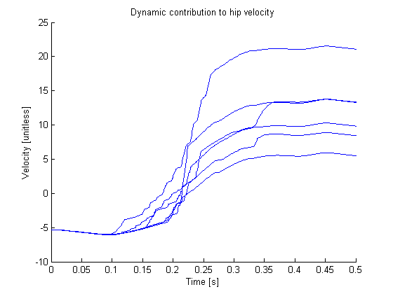
The most important outputs are:

• Hip height
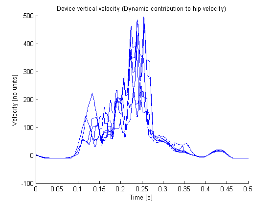
• Device y velocity, which is then subtracted from expected hip height to obtain
  • Adjusted height

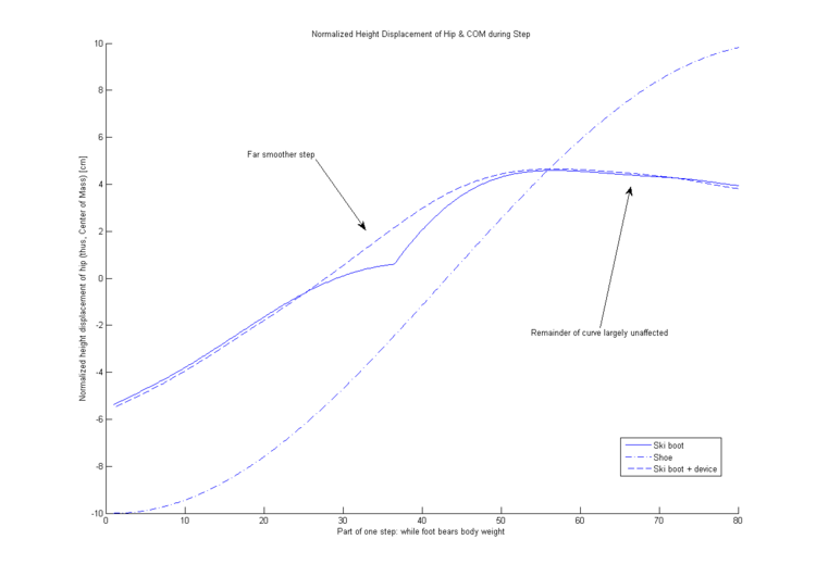
which are then compared with the ideal motion as shown in the section above. The desired product will avoid any uncomfortable periods of high ground reaction force, yet will seek to keep the hip moving in its normal sinusoidal pattern.

Hip position is then shape-compared to the ideal body motion, which is the ultimate sign of how well the device functions.

Limitations

Though this model is designed to provide a good optimization method for hip motion, it may ignore the abstract idea of "control" as felt by the user. This group does not contain a kinesiologist, so further knowledge of user feelings is not on hand. We feel that user testing will be sufficient to lay to rest any concerns about control, and that same user testing will be useful for calibration of this MATLAB model as necessary.

Also, if the motion provided in the model is extreme, the assumption of constant forward body velocity may be invalid. Again, user testing may tell how large of an effect this has. However, we feel that since foam/rubber deformation will likely be minimal compared to the vertical displacement of the body center of mass, the assumption is a valid one for now.

Results

For reference, the motion of the foot and leg during the step appears as such:

The device velocity for six different spring-damper configurations:

The device displacement for six different spring-damper configurations:

Hip height reflecting the effect of the device in different configurations:

Conclusion

• Confidence in the bulk of the results. Further refinement once actual material properties are obtained may be necessary.
• Little confidence in beginning of step, so no meaningful results there

• Need high damping, high spring in middle of step to flatten it out
• Spring/damping not a huge concern during first third of step, so save weight there
• Toe needs to be rather stiff, or be reshaped to a higher initial height

Additional conclusions as to specific material selections will surface once material properties are obtained and available for input into this model.